41 excel pie chart add labels

How to add data labels from different column in an Excel chart? Right click the data series in the chart, and select Add Data Labels > Add Data Labels from the context menu to add data labels. 2. Click any data label to select all data labels, and then click the specified data label to select it only in the chart. 3. Pie Chart in Excel - Inserting, Formatting, Filters, Data Labels To insert a Pie Chart, follow these steps:- Select the range of cells A1:B7 Go to Insert tab. In the charts group, Select the pie chart button Click on pie chart in 2D chart section. Adding Data Labels The default pie chart inserted in the above section is:-

Add data labels and callouts to charts in Excel 365 - EasyTweaks.com Step #2: When you select the "Add Labels" option, all the different portions of the chart will automatically take on the corresponding values in the table that you used to generate the chart. The values in your chat labels are dynamic and will automatically change when the source value in the table changes. Step #3: Format the data labels.

Excel pie chart add labels

Edit titles or data labels in a chart - support.microsoft.com On a chart, click the label that you want to link to a corresponding worksheet cell. On the worksheet, click in the formula bar, and then type an equal sign (=). Select the worksheet cell that contains the data or text that you want to display in your chart. You can also type the reference to the worksheet cell in the formula bar. How to Create Pie Charts in Excel (In Easy Steps) 1. Select the range A1:D2. 2. On the Insert tab, in the Charts group, click the Pie symbol. 3. Click Pie. Result: 4. Click on the pie to select the whole pie. Click on a slice to drag it away from the center. Result: Note: only if you have numeric labels, empty cell A1 before you create the pie chart. [SOLVED] Pie Chart Data Labels - Excel Help Forum No, the chart tool add-ins only have to be installed on the machine in which you are working to add the labels. I forgot to add another way to customize data labels . . . You can also click inside of the individual data label and then add a reference to a cell. For example, you can click inside of the

Excel pie chart add labels. How to create a Titled and Labeled Excel Pie Chart with C# If the Legend is only a Legend in its Own Mind. If labeling the pie pieces is enough, and you don't need the legend, you can add this line of code to prevent the legend from displaying: C#. Copy Code. chart.HasLegend = false; I recently discovered Spreadsheet Light, which seems to greatly simplify and elegantize the creation of Excel ... Committee Pie Charts The Rows button must be selected, indicating "series in" rows. The pie chart (see above) can be edited in the Chart Options window and in the completed chart by right-clicking the labels and selecting "Format Data Labels." Similarly, to display the four categories of the committee of 1697, create a new worksheet in Excel. How to Create and Format a Pie Chart in Excel - Lifewire To add data labels to a pie chart: Select the plot area of the pie chart. Right-click the chart. Select Add Data Labels . Select Add Data Labels. In this example, the sales for each cookie is added to the slices of the pie chart. How To Show Data Labels In Excel Chart - gfecc.org How To Hide Zero Data Labels In Chart In Excel; Add Or Remove Data Labels In A Chart Office Support; Display Customized Data Labels On Charts Graphs; Data Labels Projectwoman Com; Excel Charts Add Title Customize Chart Axis Legend And; Change The Format Of Data Labels In A Chart Office Support; How To Insert Data Labels To A Pie Chart In Excel ...

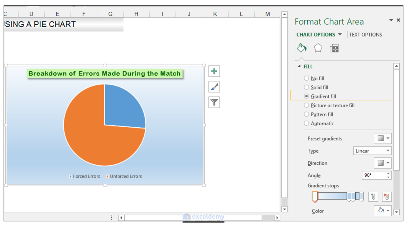
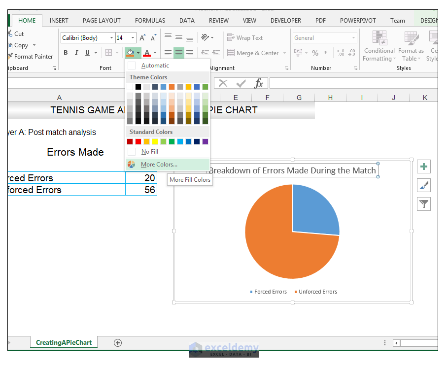
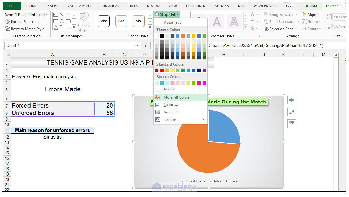
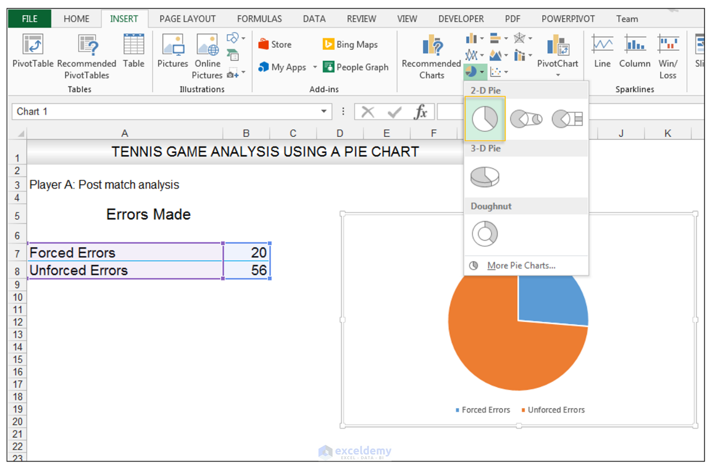
How to Make a Pie Chart in Excel & Add Rich Data Labels to The Chart! Creating and formatting the Pie Chart 1) Select the data. 2) Go to Insert> Charts> click on the drop-down arrow next to Pie Chart and under 2-D Pie, select the Pie Chart, shown below. 3) Chang the chart title to Breakdown of Errors Made During the Match, by clicking on it and typing the new title. How to display leader lines in pie chart in Excel? - ExtendOffice To display leader lines in pie chart, you just need to check an option then drag the labels out. 1. Click at the chart, and right click to select Format Data Labels from context menu. 2. In the popping Format Data Labels dialog/pane, check Show Leader Lines in the Label Options section. See screenshot: 3. Close the dialog, now you can see some leader lines appear. If you want to show all leader lines, just drag the labels out of the pie one by one. c# - Add data labels to excel pie chart - Stack Overflow private void drawfractionchart (excel.worksheet activesheet, excel.chartobjects xlcharts, excel.range xrange, excel.range yrange) { excel.chartobject mychart = (excel.chartobject)xlcharts.add (200, 500, 200, 100); excel.chart chartpage = mychart.chart; excel.seriescollection seriescollection = chartpage.seriescollection (); excel.series … Pie chart data labels not updating! | MrExcel Message Board Pie data label updating OK, I just tried it on a workbook of smaller total size and reduced formulaic complexity, and the labels all updated correctly and instantly. So now my question becomes, Is there any way to force Excel to update labels on highly complex or formulaic sheets? Thanks . . .

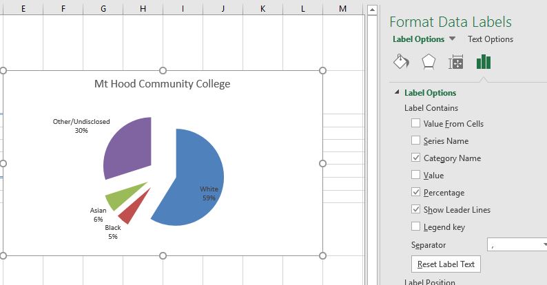
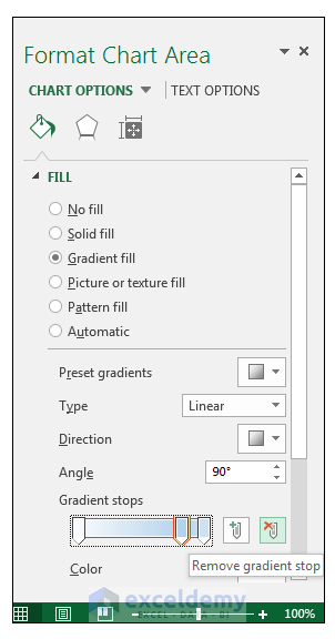
How to ☝️Make a Pie Chart in Excel (Free Template) 1. Right-click on your pie chart and pick " Format Data Series " from the menu that appears. 2. Go to the " Series Option " tab. 3. Set the " Angle of first slice " value to " 90° " to rotate the chart 90 degrees clockwise - and the great news is that you can tweak the value however you want. How to Make a PIE Chart in Excel (Easy Step-by-Step Guide) Here are the steps to format the data label from the Design tab: Select the chart. This will make the Design tab available in the ribbon. In the Design tab, click on the Add Chart Element (it's in the Chart Layouts group). Hover the cursor on the Data Labels option. Adding data labels to a pie chart - Excel General - OzGrid Re: Adding data labels to a pie chart To include the percentages: Code .ApplyDataLabels Type:=xlDataLabelsShowLabelAndPercent I don't know how you will get them bold. Why not try recording a macro when you do that manually? That's how I found the code to show the labels. Just found it: Code .SeriesCollection (1).DataLabels.Font.FontStyle = "Bold" Inserting Data Label in the Color Legend of a pie chart Inserting Data Label in the Color Legend of a pie chart. Hi, I am trying to insert data labels (percentages) as part of the side colored legend, rather than on the pie chart itself, as displayed on the image below. Does Excel offer that option and if so, how can i go about it?

How to Make a Pie Chart in Excel & Add Rich Data Labels to The Chart!

How can I add labels with percentage to a pie chart in Python? And this is my Excel file: Location Country Revenue Loc1 China 23 Loc2 China 48 Loc3 Netherlands 17 Loc4 Germany 21 What I want to do, is to add labels with percentage inside the pie chart and to keep my labels with the countries.

Excel Chapter 2 – Business Computers 365

Pie Chart in Excel | How to Create Pie Chart - EDUCBA Step 1: Select the data to go to Insert, click on PIE, and select 3-D pie chart. Step 2: Now, it instantly creates the 3-D pie chart for you. Step 3: Right-click on the pie and select Add Data Labels. This will add all the values we are showing on the slices of the pie.

How to insert data labels to a Pie chart in Excel 2013 - YouTube

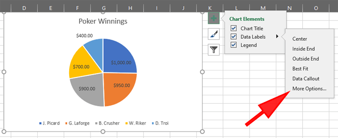
Add or remove data labels in a chart - support.microsoft.com Add data labels to a chart Click the data series or chart. To label one data point, after clicking the series, click that data point. In the upper right corner, next to the chart, click Add Chart Element > Data Labels. To change the location, click the arrow, and choose an option. If you want to ...

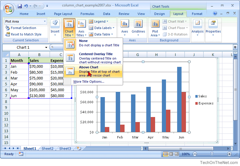
MS Excel 2007: How to Create a Column Chart

excel - Pie Chart VBA DataLabel Formatting - Stack Overflow sub updatechartformat () with activesheet.chartobjects ("chart 4") .activate with .chart.seriescollection (1).datalabels .showpercentage = true .separator = "" & chr (10) & "" end with end with with activesheet.chartobjects ("chart 1") .activate with .chart.seriescollection (1).datalabels .showpercentage = true .showvalue = false …

How to Create Multi-Category Chart in Excel - Excel Board

Chart.ApplyDataLabels method (Excel) | Microsoft Docs The type of data label to apply. True to show the legend key next to the point. The default value is False. True if the object automatically generates appropriate text based on content. For the Chart and Series objects, True if the series has leader lines. Pass a Boolean value to enable or disable the series name for the data label.

4.1 Choosing a Chart Type – Beginning Excel, First Edition

How to Create a Pie Chart in Excel | Smartsheet Enter data into Excel with the desired numerical values at the end of the list. Create a Pie of Pie chart. Double-click the primary chart to open the Format Data Series window. Click Options and adjust the value for Second plot contains the last to match the number of categories you want in the "other" category.

How to Make a Pie Chart in Excel & Add Rich Data Labels to The Chart!

Microsoft Excel Tutorials: Add Data Labels to a Pie Chart To add the numbers from our E column (the viewing figures), left click on the pie chart itself to select it: The chart is selected when you can see all those blue circles surrounding it. Now right click the chart. You should get the following menu: From the menu, select Add Data Labels. New data labels will then appear on your chart:

EXCEL Charts: Column, Bar, Pie and Line

Pie of Pie Chart in Excel - Inserting, Customizing, Formatting To insert a Pie of Pie chart:- Select the data range A1:B7. Enter in the Insert Tab. Select the Pie button, in the charts group. Select Pie of Pie chart in the 2D chart section. Adding Data Labels to Pie of Pie Chart The chart inserted in the above section is:-

Microsoft Excel Tutorials: Add Data Labels to a Pie Chart

Adding data labels to a Pie Chart in VBA - Automate Excel VBA Code Examples for Excel. Excel. Formula Tutorials; Functions List. Excel Formulas Examples List. Excel Boot Camp. Shortcuts. Shortcut Training App; List of Shortcuts; Shortcut Coach. Charts. Chart Templates; Chart Add-in; Charts List; Excel VBA Consulting - Get Help & Hire an Expert!

How to Create and Label a Pie Chart in Excel 2013 : 8 Steps - Instructables

Creating Pie Chart and Adding/Formatting Data Labels (Excel) Creating Pie Chart and Adding/Formatting Data Labels (Excel)

Excel Charts: Excel Pie Chart With Individual Slice Radius

[SOLVED] Pie Chart Data Labels - Excel Help Forum No, the chart tool add-ins only have to be installed on the machine in which you are working to add the labels. I forgot to add another way to customize data labels . . . You can also click inside of the individual data label and then add a reference to a cell. For example, you can click inside of the

How to Make a Pie Chart - ExcelNotes

How to Create Pie Charts in Excel (In Easy Steps) 1. Select the range A1:D2. 2. On the Insert tab, in the Charts group, click the Pie symbol. 3. Click Pie. Result: 4. Click on the pie to select the whole pie. Click on a slice to drag it away from the center. Result: Note: only if you have numeric labels, empty cell A1 before you create the pie chart.