43 how to show labels in excel chart
Excel charts: how to move data labels to legend - Microsoft Tech Community @Matt_Fischer-Daly . You can't do that, but you can show a data table below the chart instead of data labels: Click anywhere on the chart. On the Design tab of the ribbon (under Chart Tools), in the Chart Layouts group, click Add Chart Element > Data Table > With Legend Keys (or No Legend Keys if you prefer) How to show values in data labels of Excel Pareto Chart when chart is ... I've made the chart using the first worksheet column for category labels, the second for the bars (percentages), and the third for the line cumulative percentages). I added data labels to the bars, using Excel 2013's option to use label text from cells, referencing the text in the fourth worksheet column.
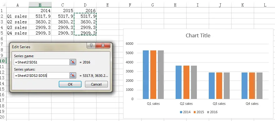
Dynamically Label Excel Chart Series Lines - My Online Training Hub Step 1: Duplicate the Series. The first trick here is that we have 2 series for each region; one for the line and one for the label, as you can see in the table below: Select columns B:J and insert a line chart (do not include column A). To modify the axis so the Year and Month labels are nested; right-click the chart > Select Data > Edit the ...
How to show labels in excel chart
Excel charts: add title, customize chart axis, legend and data labels ... Click anywhere within your Excel chart, then click the Chart Elements button and check the Axis Titles box. If you want to display the title only for one axis, either horizontal or vertical, click the arrow next to Axis Titles and clear one of the boxes: Click the axis title box on the chart, and type the text. How do I show month in Excel chart? - hizen.from-va.com Click the "Axis Options" arrow to expand the section and select "Date Axis." Click the "Base" drop-down menu and select "Months."The graph then uses months, but the labels use specific and potentially inaccurate dates.Click "Number" to expand the section, click the "Category" drop-down menu and choose "Custom." How To Add Axis Labels In Excel [Step-By-Step Tutorial] First off, you have to click the chart and click the plus (+) icon on the upper-right side. Then, check the tickbox for 'Axis Titles'. If you would only like to add a title/label for one axis (horizontal or vertical), click the right arrow beside 'Axis Titles' and select which axis you would like to add a title/label. Editing the Axis Titles
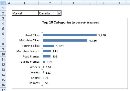
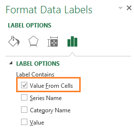
How to show labels in excel chart. How to Insert Axis Labels In An Excel Chart | Excelchat We will go to Chart Design and select Add Chart Element Figure 6 – Insert axis labels in Excel In the drop-down menu, we will click on Axis Titles, and subsequently, select Primary vertical Figure 7 – Edit vertical axis labels in Excel Now, we can enter the name we want for the primary vertical axis label. How to Create a Bar Chart With Labels Above Bars in Excel In the Format Data Labels pane, under Label Options selected, set the Label Position to Inside Base. 10. Then, under Label Contains, check the Category Name option and uncheck the Value and Show Leader Lines options. 11. Next, while the labels are still selected, click on Text Options, and then click on the Textbox icon. 12. Add or remove data labels in a chart - support.microsoft.com Click Label Options and under Label Contains, select the Values From Cells checkbox. When the Data Label Range dialog box appears, go back to the spreadsheet and select the range for which you want the cell values to display as data labels. When you do that, the selected range will appear in the Data Label Range dialog box. Then click OK. How to Add Labels to Scatterplot Points in Excel - Statology Step 3: Add Labels to Points. Next, click anywhere on the chart until a green plus (+) sign appears in the top right corner. Then click Data Labels, then click More Options…. In the Format Data Labels window that appears on the right of the screen, uncheck the box next to Y Value and check the box next to Value From Cells.
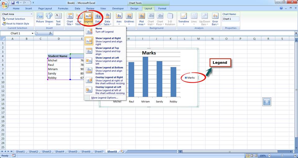
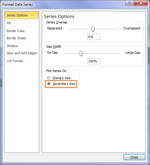
How to use data labels in a chart - YouTube Excel charts have a flexible system to display values called "data labels". Data labels are a classic example a "simple" Excel feature with a huge range of o... How To Add Data Labels In Excel - INfo Blog To format data labels in excel, choose the set of data labels to format. Source: . Use a label for flexible placement of instructions, to emphasize text, and when merged cells or a specific cell location is not a practical solution. Click the chart to show the chart elements button. Source: superuser.com How to Add Labels to Show Totals in Stacked Column Charts in Excel In the chart, right-click the "Total" series and then, on the shortcut menu, select Add Data Labels. 9. Next, select the labels and then, in the Format Data Labels pane, under Label Options, set the Label Position to Above. 10. While the labels are still selected set their font to Bold. 11. How to add or move data labels in Excel chart? In Excel 2013 or 2016. 1. Click the chart to show the Chart Elements button . 2. Then click the Chart Elements, and check Data Labels, then you can click the arrow to choose an option about the data labels in the sub menu. See screenshot: In Excel 2010 or 2007. 1. click on the chart to show the Layout tab in the Chart Tools group. See ...
How to hide zero data labels in chart in Excel? - ExtendOffice If you want to hide zero data labels in chart, please do as follow: 1. Right click at one of the data labels, and select Format Data Labels from the context menu. See screenshot: 2. In the Format Data Labels dialog, Click Number in left pane, then select Custom from the Category list box, and type #"" into the Format Code text box, and click Add button to add it to Type list box. Custom Chart Data Labels In Excel With Formulas Follow the steps below to create the custom data labels. Select the chart label you want to change. In the formula-bar hit = (equals), select the cell reference containing your chart label's data. In this case, the first label is in cell E2. Finally, repeat for all your chart laebls. How to Use Cell Values for Excel Chart Labels Mar 12, 2020 · Select the chart, choose the “Chart Elements” option, click the “Data Labels” arrow, and then “More Options.” Uncheck the “Value” box and check the “Value From Cells” box. Select cells C2:C6 to use for the data label range and then click the “OK” button. The values from these cells are now used for the chart data labels. Add a DATA LABEL to ONE POINT on a chart in Excel All the data points will be highlighted. Click again on the single point that you want to add a data label to. Right-click and select ' Add data label '. This is the key step! Right-click again on the data point itself (not the label) and select ' Format data label '. You can now configure the label as required — select the content of ...
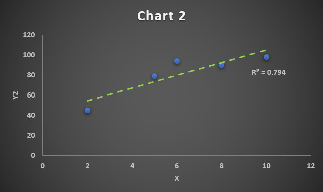
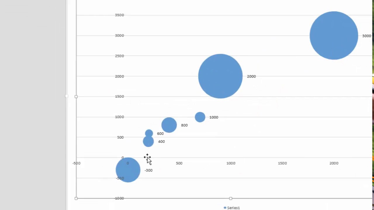
Correlation Chart in Excel - GeeksforGeeks
Edit titles or data labels in a chart - support.microsoft.com On a chart, click the label that you want to link to a corresponding worksheet cell. On the worksheet, click in the formula bar, and then type an equal sign (=). Select the worksheet cell that contains the data or text that you want to display in your chart. You can also type the reference to the worksheet cell in the formula bar.

add labels to excel chart 218253.image0 - Top Label Maker
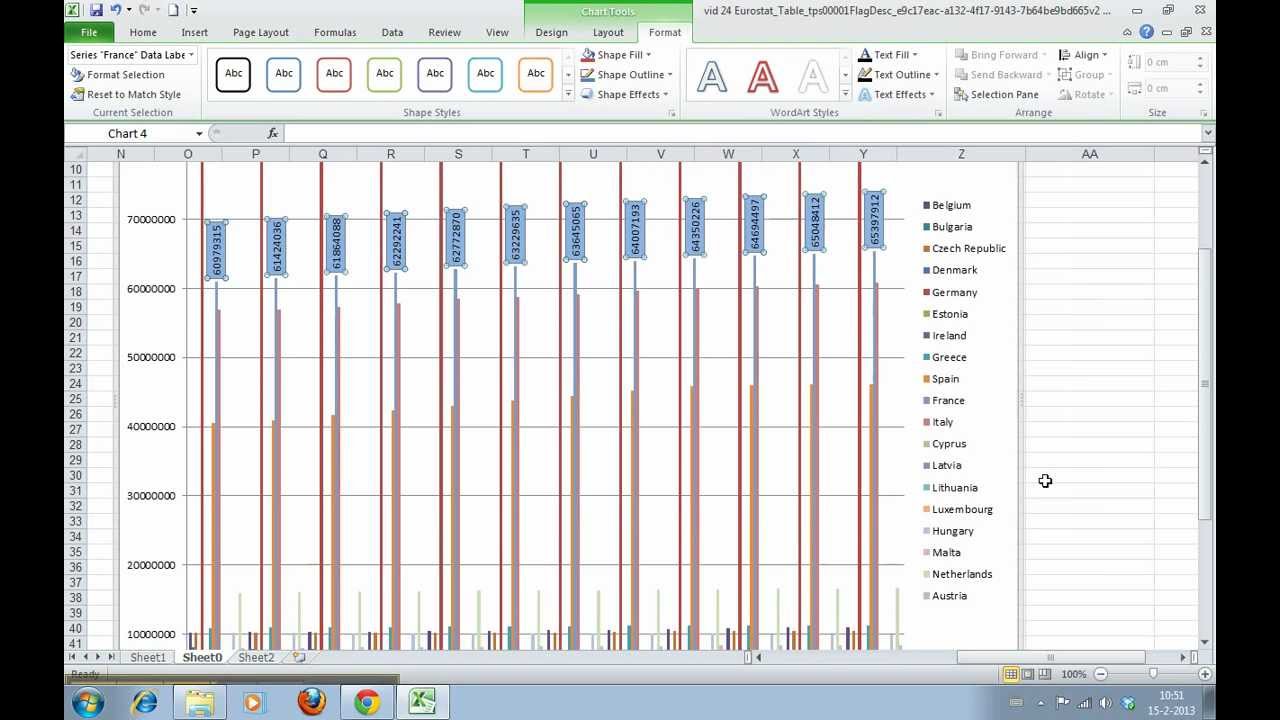
How to I rotate data labels on a column chart so that they are ... To change the text direction, first of all, please double click on the data label and make sure the data are selected (with a box surrounded like following image). Then on your right panel, the Format Data Labels panel should be opened. Go to Text Options > Text Box > Text direction > Rotate. And the text direction in the labels should be in ...
Basic Excel Chart Formatting - MS Excel Charting Tutorial Part 4 | Vertical Horizons
Excel Charts: Dynamic Label positioning of line series - XelPlus Select your chart and go to the Format tab, click on the drop-down menu at the upper left-hand portion and select Series "Budget". Go to Layout tab, select Data Labels > Right. Right mouse click on the data label displayed on the chart. Select Format Data Labels. Under the Label Options, show the Series Name and untick the Value.

How to edit the label of a chart in Excel? - Stack Overflow
How To Create A Pie Chart In Excel (With Percentages) - YouTube In this video, I'm going to show you how to create a pie chart by using Microsoft Excel. I will show you how to add data labels that are percentages and even...
How to Add Data Labels in an Excel Chart in Excel 2010 - YouTube
How to Customize Your Excel Pivot Chart Data Labels - dummies When you click the command button, Excel displays a menu with commands corresponding to locations for the data labels: None, Center, Left, Right, Above, and Below. None signifies that no data labels should be added to the chart and Show signifies heck yes, add data labels. The menu also displays a More Data Label Options command.

Nested donut chart (also known as Multi-level doughnut chart, Multi-series doughnut chart ...
How to create a chart with both percentage and value in Excel? In the Format Data Labels pane, please check Category Name option, and uncheck Value option from the Label Options, and then, you will get all percentages and values are displayed in the chart, see screenshot: 15.

How to edit the label of a chart in Excel? - Stack Overflow
How to Show Percentages in Stacked Column Chart in Excel? By default, the data labels are shown in the form of chart data Value (Image 1). But very often user needs to plot charts with actual data and show percentages/custom values on the chart instead of default data. For that we have an option "Value From Cells" in chart "Format Data Label" (Image 2) to select a custom range. Image 1 Image 2
Add Average Marker to Excel Box Plot - Box and Whisker Chart - YouTube
How to Add Percentages to Excel Bar Chart - Excel Tutorials If we would like to add percentages to our bar chart, we would need to have percentages in the table in the first place. We will create a column right to the column points in which we would divide the points of each player with the total points of all players. We will select range A1:C8 and go to Insert >> Charts >> 2-D Column >> Stacked Column ...
35 How To Add Label To Excel Chart - Labels 2021
Multiple Data Labels on bar chart? - Excel Help Forum Add label to the second serie, outside of the bar Edit separately each label, egal to % value with formula to be dynamic Set the overlap to 100% Insert title with formula Hope this helps Best regards Attached Files sample chart two data labels_jpr73.xlsx (12.1 KB, 1248 views) Download Register To Reply 01-26-2012, 11:11 AM #6 Andy Pope Forum Guru
34 How To Label A Chart In Excel - Label Ideas 2020
excel - How to not display labels in pie chart that are 0% - Stack Overflow I have some data in excel that I want to graph in a pie chart (see image 1) where the text will be the labels and the numbers will turn into percentages. The problem is, when i go to graph the data, it shows the labels for ALL of the sections, even the ones that are 0% in the pie chart. So this really overtakes my entire chart.
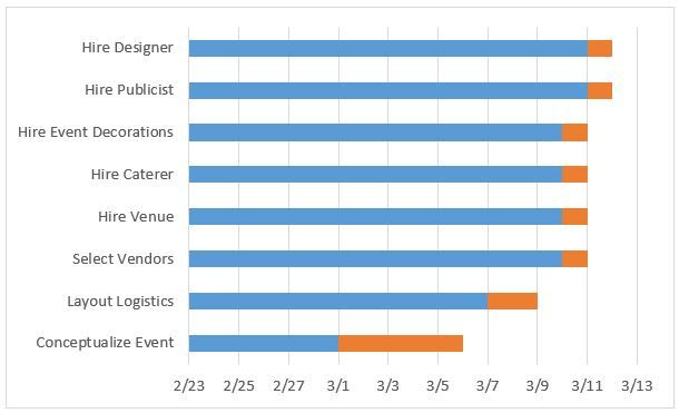
How to Create a Gantt Chart in Excel
How To Add Data Labels In Excel - WRG BLOGER When you check the box, you'll see. Click inside the chart area to display the chart tools. Source: . Select the chart, choose the "chart elements" option, click the "data labels" arrow, and then "more options.". To do this, click the "format" tab within the "chart tools" contextual tab in the ribbon.
30 How To Label A Chart In Excel - Labels Niche Ideas
How To Add Axis Labels In Excel [Step-By-Step Tutorial] First off, you have to click the chart and click the plus (+) icon on the upper-right side. Then, check the tickbox for 'Axis Titles'. If you would only like to add a title/label for one axis (horizontal or vertical), click the right arrow beside 'Axis Titles' and select which axis you would like to add a title/label. Editing the Axis Titles
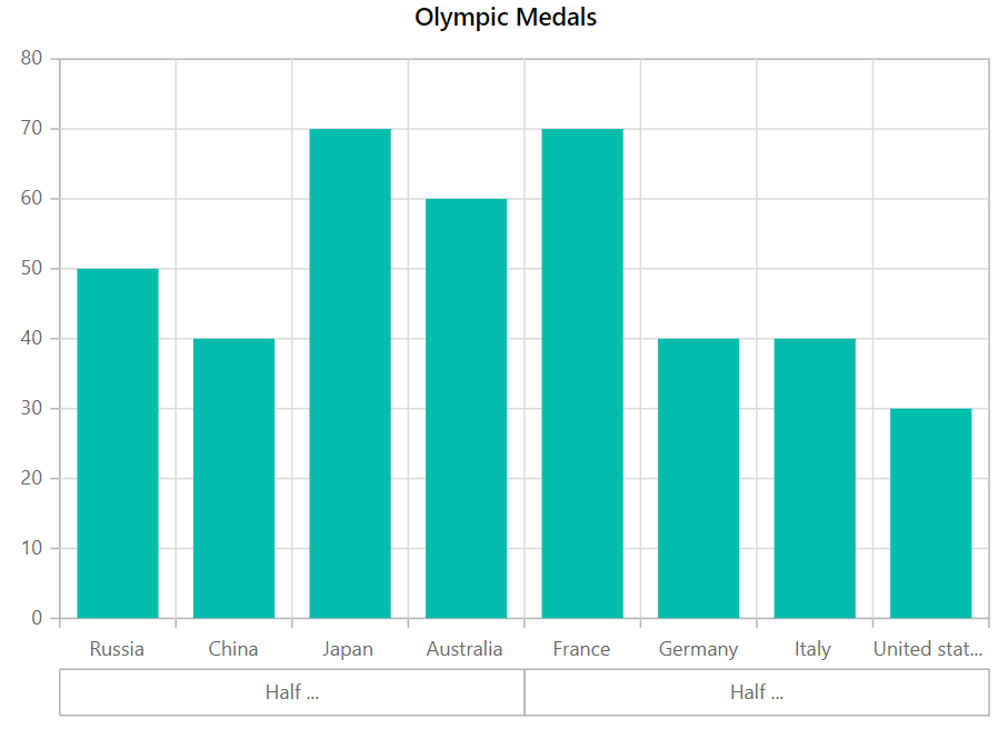
Axis Labels in Blazor Chart component - Syncfusion
How do I show month in Excel chart? - hizen.from-va.com Click the "Axis Options" arrow to expand the section and select "Date Axis." Click the "Base" drop-down menu and select "Months."The graph then uses months, but the labels use specific and potentially inaccurate dates.Click "Number" to expand the section, click the "Category" drop-down menu and choose "Custom."
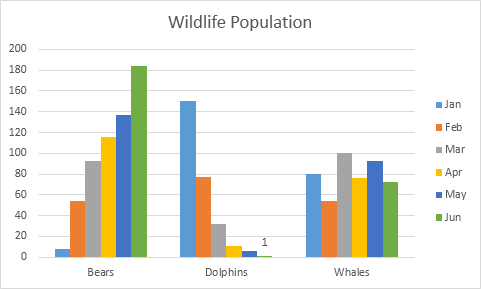
Excel clustered column chart - Access-Excel.Tips
Excel charts: add title, customize chart axis, legend and data labels ... Click anywhere within your Excel chart, then click the Chart Elements button and check the Axis Titles box. If you want to display the title only for one axis, either horizontal or vertical, click the arrow next to Axis Titles and clear one of the boxes: Click the axis title box on the chart, and type the text.

Excel - Sort Labels in a Chart - YouTube
Excel Gantt Chart - Free Excel Templates
Excel Custom Chart Labels • My Online Training Hub
Excel Custom Chart Labels • My Online Training Hub
Post a Comment for "43 how to show labels in excel chart"